Hot Start Vignette
Imports
# basic imports
import os
import pandas as pd
import numpy as np
import IPython

# tcrdist classes
from tcrdist.repertoire import TCRrep
from tcrdist.subset import TCRsubset
from tcrdist.cdr3_motif import TCRMotif
from tcrdist.storage import StoreIOMotif, StoreIOEntropy

# tcrdist functions
from tcrdist import plotting
from tcrdist.mappers import populate_legacy_fields

# scipy functions for clustering
from scipy.spatial import distance
from scipy.cluster.hierarchy import linkage, dendrogram, fcluster

# sklearn functions for low-dimensional embeddings
from sklearn.manifold import TSNE, MDS

# plotnine to allow grammar of graphics plotting akin to R's ggplot2
import plotnine as gg
TCRrep
Download repertoire data: (dash.csv 375KB).
| subject | epitope | count | v_a_gene | j_a_gene | cdr3_a_aa | cdr3_a_nucseq | v_b_gene | j_b_gene | cdr3_b_aa | cdr3_b_nucseq | clone_id |
|---|---|---|---|---|---|---|---|---|---|---|---|
| mouse_subject0050 | PA | 2 | TRAV7-3*01 | TRAJ33*01 | CAVSLDSNYQLIW | tgtgcagtgagcctcgatagcaactatcagttgatctgg | TRBV13-1*01 | TRBJ2-3*01 | CASSDFDWGGDAETLYF | tgtgccagcagtgatttcgactggggaggggatgcagaaacgctgtatttt | mouse_tcr0072.clone |
| mouse_subject0050 | PA | 6 | TRAV6D-6*01 | TRAJ56*01 | CALGDRATGGNNKLTF | tgtgctctgggtgacagggctactggaggcaataataagctgactttt | TRBV29*01 | TRBJ1-1*01 | CASSPDRGEVFF | tgtgctagcagtccggacaggggtgaagtcttcttt | mouse_tcr0096.clone |
| mouse_subject0050 | PA | 1 | TRAV6D-6*01 | TRAJ49*01 | CALGSNTGYQNFYF | tgtgctctgggctcgaacacgggttaccagaacttctatttt | TRBV29*01 | TRBJ1-5*01 | CASTGGGAPLF | tgtgctagcacagggggaggggctccgcttttt | mouse_tcr0276.clone |
Calculate pairwise TCR distances between all clones in the repertoire.
#1 load data, subset to receptors recognizing "PA" epitope
tcrdist2_df = pd.read_csv(os.path.join("dash.csv"))
tcrdist2_df = tcrdist2_df[tcrdist2_df.epitope == "PA"].copy()

#2 create instance of TCRrep class, initializes input as tr.cell_df attribute
tr = TCRrep(cell_df = tcrdist2_df, chains = ['alpha','beta'],organism = "mouse")

#3 Infer CDR1,CDR2,CDR2.5 (a.k.a. phmc) from germline v-genes
tr.infer_cdrs_from_v_gene(chain = 'alpha', imgt_aligned=True)
tr.infer_cdrs_from_v_gene(chain = 'beta',  imgt_aligned=True)

#4 Define index columns for determining unique clones.
tr.index_cols = ['clone_id', 'subject', 'epitope',
                'v_a_gene',  'j_a_gene', 'v_b_gene', 'j_b_gene',
                'cdr3_a_aa', 'cdr3_b_aa',
                'cdr1_a_aa', 'cdr2_a_aa', 'pmhc_a_aa',
                'cdr1_b_aa', 'cdr2_b_aa', 'pmhc_b_aa',
                'cdr3_b_nucseq', 'cdr3_a_nucseq']

#4 Deduplicate based on index cols, creating tr.clone_df attribute
tr.deduplicate()

#5 calculate tcrdists by method in Dash et al.
tr._tcrdist_legacy_method_alpha_beta()

#6 Check that sum of alpah-chain and beta-chain distance matrices equal paired_tcrdist
distA = tr.dist_a
distB = tr.dist_b
assert np.all(((distA + distB) - tr.paired_tcrdist) == 0)
Hier. Cluster TCR-Distances
The pairwise TCR distance matrix calculated by
tcrdist2.repertoire.TCRrep (i.e., accessible as tr.paired_tcrdist) can serve
as the input for scipy.cluster.hierarchy tools or your preferred python
library for unsupervised clustering of sequences within the repertoire.
The rows of tr.clone_df match the order of rows in
tr.paired_distance. Thus, any cluster_index you produce, must
match length and order of tr.clone_df.
from scipy.spatial import distance
from scipy.cluster.hierarchy import linkage, dendrogram, fcluster
compressed_dmat = distance.squareform(tr.paired_tcrdist, force = "vector")
Z = linkage(compressed_dmat, method = "complete")
den = dendrogram(Z, color_threshold = np.inf, no_plot = True)
cluster_index = fcluster(Z, t = 20, criterion = "maxclust")
assert len(cluster_index) == tr.clone_df.shape[0]
assert len(cluster_index) == tr.paired_tcrdist.shape[0]
tr.clone_df['cluster_index'] = cluster_index
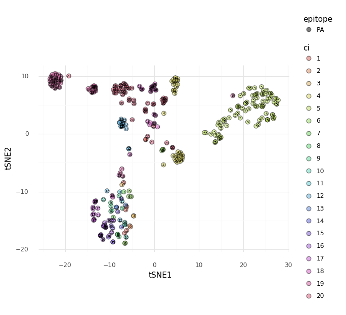
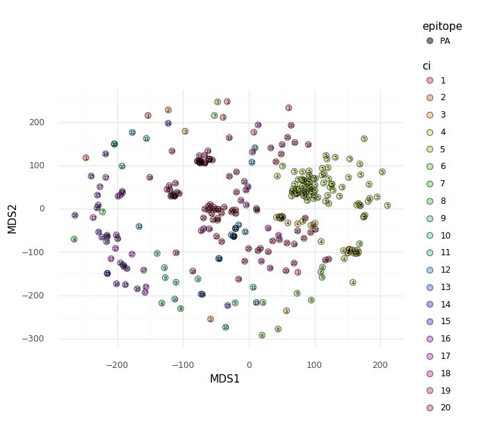
2D Embeddings
The pairwise TCR distance matrix calculated by
tcrdist2.repertoire.TCRrep (i.e., accessible as tr.paired_tcrdist) can be used
as input for embedding the pairwise dissimilarity matrix in fewer dimensions.
Here we provide an example using sklearn to perform tSNE and MDS.
import numpy as np
from sklearn.manifold import TSNE, MDS
X = tr.paired_tcrdist
X_embedded = TSNE(n_components=2).fit_transform(X)

tsne_df = pd.DataFrame(X_embedded, columns = ["tSNE1","tSNE2"])
tsne_df['ci'] = cluster_index
tsne_df['ci'] = tsne_df['ci'].astype('category')
tsne_df['epitope'] = tr.clone_df.epitope.astype('category')

X_embedded_mds = MDS(n_components=2, dissimilarity='precomputed').fit_transform(X)
mds_df = pd.DataFrame(X_embedded_mds, columns = ["MDS1","MDS2"])
mds_df['ci'] = cluster_index
mds_df['ci'] = mds_df['ci'].astype('category')
mds_df['epitope'] = tr.clone_df.epitope.astype('category')
def gg_embed_plot(df,
                  xvar = 'tSNE1',
                  yvar = 'tSNE2'):
    """
    Function for plotting embedding using plotnine

    Parameters
    ----------
    df   : pandas.DataFrame
    xvar : str
        column with data to be plotted along the x-axis
    yvar : str
        column with data to be plotted along the y-axis

    Returns
    -------
    gg_em_plot : plotnine.ggplot.ggplot

    """
    import plotnine as gg

    gg_em_plt = ( gg.ggplot(df)
                + gg.aes(x = xvar,
                         y = yvar,
                         col = "ci",
                         label = 'ci',
                         fill = "ci",
                         shape = "epitope")
                + gg.geom_point(size = 3, alpha = .5)
                + gg.geom_text(size = 5)
                + gg.theme_minimal())

    return(gg_em_plt)
TCRsubset
Consider cluster 5 of the PA-reactive repertoire in the plot above. Using tcrdist2 we can search
for motifs in any portion of the repertoire by specifying a criteria and initializing
TCRsubset with a subset of the data as shown below.
# define a logical criteria
criteria = (cluster_index == 5)

# subset the TCRrep clone DataFrame to only those sequences meeting that criteria
clone_df_subset = tr.clone_df[criteria]
clone_df_subset = clone_df_subset[clone_df_subset.epitope == "PA"].copy()

# subset the alpha chain and beta chain distance matrices using the `clone_df_subset.clone_id` index
dist_a_subset = tr.dist_a.loc[clone_df_subset.clone_id, clone_df_subset.clone_id].copy()
dist_b_subset = tr.dist_b.loc[clone_df_subset.clone_id, clone_df_subset.clone_id].copy()

# use the populate_legacy_fields function to add some columns needed for compatability with tcrdist1
clone_df_subset = populate_legacy_fields(df = clone_df_subset, chains =['alpha', 'beta'])

# initialize an instance of the TCRsubset class.
ts = TCRsubset(clone_df_subset,
            organism = "mouse",
            epitopes = ["PA"] ,
            epitope = "PA",
            chains = ["A","B"],
            dist_a = dist_a_subset,
            dist_b = dist_b_subset)
read 169087 A-chains from /Users/kmayerbl/TCRDIST/tcrdist2/tcrdist/db/alphabeta_db.tsv_files/new_nextgen_chains_mouse_A.tsv
read 1947545 B-chains from /Users/kmayerbl/TCRDIST/tcrdist2/tcrdist/db/alphabeta_db.tsv_files/new_nextgen_chains_mouse_B.tsv
Plot Gene Usage
Gene Usage in the Repertoire
Consider the gene usage of the whole PA-reactive repertoire.
from tcrdist import plotting
gene_usage_repertoire_svg = plotting.plot_pairings(cell_df = tr.clone_df,
                                        cols = ['j_a_gene',
                                                'v_a_gene',
                                                'v_b_gene',
                                                'j_b_gene'],
                                        count_col='count')
IPython.display.SVG(data=gene_usage_repertoire_svg)

Gene Usage in the Subset
Consider the gene usage in cluster 5 of the PA-reactive repertoire.
gene_usage_subset_svg = plotting.plot_pairings(cell_df = ts.clone_df,
                                        cols = ['j_a_gene',
                                                'v_a_gene',
                                                'v_b_gene',
                                                'j_b_gene'],
                                        count_col='count')

IPython.display.SVG(data=gene_usage_subset_svg)

Discover Motifs
This process may take a few minutes depending on the size of the cluster selected.
if os.path.isfile("dash_PA_cluster_5_motifs.csv"):
    ts.motif_df = pd.read_csv("dash_PA_cluster_5_motifs.csv")
else:
    motif_df = ts.find_motif()
Save Discovered Motifs
ts.motif_df.to_csv("dash_PA_cluster_5_motifs.csv", index = False)
Plot Motifs
motif_list_a = list()
motif_logos_a = list()
for i,row in ts.motif_df[ts.motif_df.ab == "A"].iterrows():
    StoreIOMotif_instance = ts.eval_motif(row)
    motif_list_a.append(StoreIOMotif_instance)
    motif_logos_a.append(plotting.plot_pwm(StoreIOMotif_instance, create_file = False, my_height = 200, my_width = 600))

motif_list_b = list()
motif_logos_b = list()
for i,row in ts.motif_df[ts.motif_df.ab == "B"].iterrows():
    StoreIOMotif_instance = ts.eval_motif(row)
    motif_list_b.append(StoreIOMotif_instance)
    motif_logos_b.append(plotting.plot_pwm(StoreIOMotif_instance, create_file = False, my_height = 200, my_width = 600))
Top Alpha-Chain Motif
You can visualize the ith motifs by changing the index [0] to [i] in the code below.
IPython.display.SVG(motif_logos_a[0])


All Code in One Block
# All code in one block, minus plotting.

# basic imports
import os
import pandas as pd
import numpy as np
import IPython

# tcrdist classes
from tcrdist.repertoire import TCRrep
from tcrdist.subset import TCRsubset
from tcrdist.cdr3_motif import TCRMotif
from tcrdist.storage import StoreIOMotif, StoreIOEntropy

# tcrdist functions
from tcrdist import plotting
from tcrdist.mappers import populate_legacy_fields

# scipy functions for clustering
from scipy.spatial import distance
from scipy.cluster.hierarchy import linkage, dendrogram, fcluster

# sklearn functions for low-dimensional embeddings
from sklearn.manifold import TSNE, MDS

# plotnine to allow grammar of graphics plotting akin to R's ggplot2
import plotnine as gg

#1 load data, subset to receptors recognizing "PA" epitope
tcrdist2_df = pd.read_csv(os.path.join("tcrdist",""test_files_compact","dash.csv"))
tcrdist2_df = tcrdist2_df[tcrdist2_df.epitope == "PA"].copy()

#2 create instance of TCRrep class, initializes input as tr.cell_df attribute
tr = TCRrep(cell_df = tcrdist2_df, chains = ['alpha','beta'],organism = "mouse")

#3 Infer CDR1,CDR2,CDR2.5 (a.k.a. phmc) from germline v-genes
tr.infer_cdrs_from_v_gene(chain = 'alpha', imgt_aligned=True)
tr.infer_cdrs_from_v_gene(chain = 'beta',  imgt_aligned=True)

#4 Define index columns for determining unique clones.
tr.index_cols = ['clone_id', 'subject', 'epitope',
                'v_a_gene',  'j_a_gene', 'v_b_gene', 'j_b_gene',
                'cdr3_a_aa', 'cdr3_b_aa',
                'cdr1_a_aa', 'cdr2_a_aa', 'pmhc_a_aa',
                'cdr1_b_aa', 'cdr2_b_aa', 'pmhc_b_aa',
                'cdr3_b_nucseq', 'cdr3_a_nucseq']

#4 Deduplicate based on index cols, creating tr.clone_df attribute
tr.deduplicate()

#5 calculate tcrdists by method in Dash et al.
tr._tcrdist_legacy_method_alpha_beta()

#6 Check that sum of alpah-chain and beta-chain distance matrices equal paired_tcrdist
distA = tr.dist_a
distB = tr.dist_b
assert np.all(((distA + distB) - tr.paired_tcrdist) == 0)


# Cluster
from scipy.spatial import distance
from scipy.cluster.hierarchy import linkage, dendrogram, fcluster
compressed_dmat = distance.squareform(tr.paired_tcrdist, force = "vector")
Z = linkage(compressed_dmat, method = "complete")
den = dendrogram(Z, color_threshold = np.inf, no_plot = True)
cluster_index = fcluster(Z, t = 20, criterion = "maxclust")
assert len(cluster_index) == tr.clone_df.shape[0]
assert len(cluster_index) == tr.paired_tcrdist.shape[0]
tr.clone_df['cluster_index'] = cluster_index

# Subset to Cluster 5
criteria = (cluster_index == 5)
clone_df_subset = tr.clone_df[criteria]
clone_df_subset = clone_df_subset[clone_df_subset.epitope == "PA"].copy()
dist_a_subset = tr.dist_a.loc[clone_df_subset.clone_id, clone_df_subset.clone_id].copy()
dist_b_subset = tr.dist_b.loc[clone_df_subset.clone_id, clone_df_subset.clone_id].copy()

clone_df_subset = populate_legacy_fields(df = clone_df_subset, chains =['alpha', 'beta'])

ts = TCRsubset(clone_df_subset,
            organism = "mouse",
            epitopes = ["PA"] ,
            epitope = "PA",
            chains = ["A","B"],
            dist_a = dist_a_subset,
            dist_b = dist_b_subset)

# Find Motifs
if os.path.isfile("dash_PA_cluster_5_motifs.csv"):
    ts.motif_df = pd.read_csv("dash_PA_cluster_5_motifs.csv")
else:
    motif_df = ts.find_motif()

# Save Motifs
ts.motif_df.to_csv("dash_PA_cluster_5_motifs.csv", index = False)

# Preprocess Motifs
motif_list_a = list()
motif_logos_a = list()
for i,row in ts.motif_df[ts.motif_df.ab == "A"].iterrows():
    StoreIOMotif_instance = ts.eval_motif(row)
    motif_list_a.append(StoreIOMotif_instance)
    motif_logos_a.append(plotting.plot_pwm(StoreIOMotif_instance, create_file = False, my_height = 200, my_width = 600))

motif_list_b = list()
motif_logos_b = list()
for i,row in ts.motif_df[ts.motif_df.ab == "B"].iterrows():
    StoreIOMotif_instance = ts.eval_motif(row)
    motif_list_b.append(StoreIOMotif_instance)
    motif_logos_b.append(plotting.plot_pwm(StoreIOMotif_instance, create_file = False, my_height = 200, my_width = 600))