Detailed Example
The data for this example come from the paper “Quantifiable predictive features define epitope-specific T cell receptor repertoires” by Dash and colleagues (2017) doi:10.1038/nature22383. The CDR3 alpha and beta sequences and V and J gene usage can be downloaded from the vdjDB.
Data from this study were selected from the vdjDB using the search filter (references == PMID:28636592). This query returns data for 2442 paired alpha/beta T cell receptors from human and mouse subjects with predicted epitope specificities.
Compute Hamming Distances for Paired Alpha/Beta Chains
Data were downloaded as a tab separated flat file (vdjDB_PMID28636592.tsv).
The application programming interface for tcrdist2 involves step-wise
commands using the tcrdist.repertoire.TCRrep class, which
stores input data, methods, user-parameters, and results.
Before explaining steps and method options in detail, it is useful to present these steps as a block of code needed to calculate the ‘tcrdistances’ – weighted pairwise distance measures based on comparison across multiple T cell receptor complementarity-determining regions (CDRs) – between all mouse T cell clones in the Dash et al. 2017 dataset.
Numbered annotations describe each step. We then elaborate on alternative analysis options.
import pandas as pd
import tcrdist as td
from tcrdist import mappers
from tcrdist.repertoire import TCRrep


pd_df = pd.read_csv("vdjDB_PMID28636592.tsv", sep = "\t")      # 1
t_df = td.mappers.vdjdb_to_tcrdist2(pd_df = pd_df)              # 2
t_df.organism.value_counts                                      # 3
index_mus = t_df.organism == "MusMusculus"                      # 4
t_df_mus = t_df.loc[index_mus,:].copy()                         # 5


tr = TCRrep(cell_df = t_df_mus, organism = "mouse")             # 6

tr.infer_cdrs_from_v_gene(chain = 'alpha')                      # 7

tr.infer_cdrs_from_v_gene(chain = 'beta')                       # 8

tr.index_cols =['epitope',                                      # 9
                'subject',
                'cdr3_a_aa',
                'cdr1_a_aa',
                'cdr2_a_aa',
                'pmhc_a_aa',
                'cdr3_b_aa',
                'cdr1_b_aa',
                'cdr2_b_aa',
                'pmhc_b_aa']

tr.deduplicate()                                                # 10


tr.compute_pairwise_all(chain = "alpha",                        # 11
                        metric = "hamming",
                        processes = 6)

tr.compute_pairwise_all(chain = "beta",                         # 12
                        metric = "hamming",
                        processes = 6)

tr.compute_paired_tcrdist(chains = ['alpha','beta'],            # 13
                          replacement_weights= {'cdr3_a_aa_pw': 3,
                                                'cdr3_b_aa_pw': 3})
Stepwise Explanation
Read the .tsv data file into a pandas DataFrame.
Call
tcrdist.mappers.vdjdb_to_tcrdist2()to select and rename the appropriate columns. You are encouraged to compare the raw and tcrdist2 formatted inputspd_df.head() t_df.head()
Examine instances of human and mouse sequences in the data.
Index the sequences that come from MusMusculus (mouse).
Create a copy of the subset DataFrame t_df, including only mouse TCRs: t_df_mus.
Create an instance of the
tcrdist.repertoire.TCRrepclass initialized with the t_df_mus DataFrame.- Upon initialization, the
organismargument must be set to “mouse” - The data is now stored as
tcrdist.repertoire.TCRrep.cell_df.
tr.cell_df.head()
- Upon initialization, the
Use
tcrdist.repertoire.TCRrep.infer_cdrs_from_v_gene()to populate CDR1, CDR2 and pMHC loop fields.chainargument is set to either ‘alpha’, ‘beta’, ‘delta’, ‘gamma’
- Repeat step 7, with
chainset to ‘beta’. - Because of hypermutation occurs in the CDR3 region, the CDR3 sequence must be directly supplied. However, for the other complementarity-determining regions the sequence come form germline and are not provided in the vdjDB data product. Therefore, tcrdist2 uses the predicted v-gene variant call (i.e TRAV1-1*01) to infer the amino acid sequence at the remaining complementarity-determining regions: CDR1, CDR2, and the pMHC loop positions (the pMHC loop is between the CDR2 and CDR3).
- Repeat step 7, with
Specify index columns. Any sequence identical across all the index columns will be grouped at the following step. The count field keeps track of the number of identical clones (which may occur during clonal expansion)
Call
tcrdist.repertoire.TCRrep.deduplicate()to remove duplicates and create thetcrdist.repertoire.TCRrep.clone_dfDataFrame. - Even if there are no duplicates this step is necessary to produce the :py:obj:`tcrdist.repertoire.TCRrep.clone_df` DataFrame. - Any row of the DataFrame missing any of the CDRs specified in the index_col list will not be included in thetcrdist.repertoire.TCRrep.clone_dfDataFrame. Theclone_dfdata is now stored:tr.clone_df.head()
Call
tcrdist.repertoire.TCRrep.compute_pairwise_all()specifying the chain, metric, and number of parallel processes to use- chain argument is set to either ‘alpha’, ‘beta’, ‘delta’, ‘gamma’
- metric argument is set to either ‘hamming’, ‘nw’ or ‘custom’ In this first example we are using the Hamming Distance, which is the number of mismatching positions between two aligned strings. In a later example, we will demonstrate how tcrdist2 can incorporate amino acid substitution matrices in calculating a distance score.
- processes specified the number of available CPUs. tcrdist2 uses python’s multiprocessing package to parallelize pairwise distance computation.
Repeat the previous step setting chain argument to ‘beta’.
Call
tcrdist.repertoire.TCRrep.compute_paired_tcrdist()to compute the ‘tcrdist’- a weighted sum of the Hamming Distances at each CDR.- The argument replacement_weights takes a dictionary which specifies greater weight on sequence differences occurring in certain CDRs. (By default all CDRs are weighted equally.)
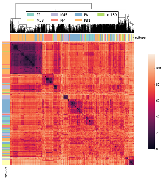
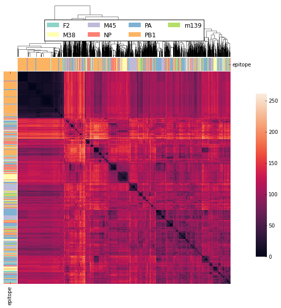
That’s it! If you’ve followed along you’ve computed over 2,000,000 tcrdists from real data in later examples we will show how tcrdist2 permits customization on this general workflow. The python code for producing the clustered Heatmap figure shown above directly from this tcrdist2 output is shown at the end of this section.
We now examine some of the flexibility of the tcrdist2 workflow.
Accessing Individual CDR Results
In the introductory workflow, we combined the number of mismatches between 8 total CDRs and combined the results into a single distance metric.
The individual Hamming Distances between CDRs is readily available within the
instance of the tcrdist.repertoire.TCRrep class.
A common naming convention is used to store a number of objects within the TCRrep class.
TCRrep.[cdr1|cdr2|cdr3|pmhc]_[a|b|d|g]_aa_pw
- the first position references the CDR.
- the second position references a: alpha, b: beta, d: delta, g: gamma chains
- the third position references the molecular type aa: amino acid or nuc: nucleotide
- the final position reference the object pw: pairwise, sm: substitution matrix, etc.
For example, the pairwise results for the alpha chain cdr3 region can be directly accessed:
tr.cdr3_a_aa_pw
The pairwise results for the beta chain cdr1 region can be directly accessed:
tr.cdr1_b_aa_pw
One could calculate a weighted tcrdist directly:
1 * tr.cdr1_b_aa_pw + 3 * tr.cdr3_a_aa_pw + 3 * tr.cdr3_b_aa_pw
But it is more practical to recalculate tcrdistances by
setting the CDR weights in the function call by passing a dictionary to the
replacement_weights argument.
Note that by default (and when store_result = True) each result is cached in
the tcrdist.repertoire.TCRrep.stored_tcrdist list.
By default, the most recently generated tcrdist is stored as
tcrdist.repertoire.TCRrep.paired_tcrdist
The following example illustrates the point.
Using Custom Weights and Stored Results
# 1
tcrdist0 = tr.compute_paired_tcrdist(chains = ['alpha','beta'],
                                     store_result = True)

replacement_weights = {'cdr1_a_aa_pw':1,
                       'cdr2_a_aa_pw':1,
                       'cdr3_a_aa_pw':2,
                       'pmhc_a_aa_pw':1,
                       'cdr1_b_aa_pw':2,
                       'cdr2_b_aa_pw':2,
                       'cdr3_b_aa_pw':4,
                       'pmhc_b_aa_pw':0}
# 2
tcrdist1 = tr.compute_paired_tcrdist(chains = ['alpha','beta'],
                        replacement_weights= replacement_weights,
                        store_result = True)

# 3
tr.stored_tcrdist[0]
tr.stored_tcrdist[1]
Repeat step 13 from the previous example using the default weights of 1
Repeat step 13 using new weights.
Access a stored result. The weights are stored along with the pairwise distances.
- {‘paired_tcrdist’: array([[ 0., 76., 80., …, 89., 89., 87.],
[ 76., 0., 60., …, 81., 75., 43.], [ 80., 60., 0., …, 59., 81., 77.], …, [ 89., 81., 59., …, 0., 60., 58.], [ 89., 75., 81., …, 60., 0., 40.], [ 87., 43., 77., …, 58., 40., 0.]]),
- ‘paired_tcrdist_weights’: {‘cdr1_a_aa_pw’: 1,
‘cdr1_b_aa_pw’: 2, ‘cdr2_a_aa_pw’: 1, ‘cdr2_b_aa_pw’: 2, ‘cdr3_a_aa_pw’: 2, ‘cdr3_b_aa_pw’: 4, ‘pmhc_a_aa_pw’: 1, ‘pmhc_b_aa_pw’: 2}}
Computing Distances with Substitution Matrices
The introductory example used the Hamming Distance (number of aligned positions with mismatching information) to calculate pairwise distance between each receptor.
Another approach is to use reciprocal Needleman-Wunsch alignment scores.
In this case, metric is set to “nw” for
tcrdist.repertoire.TCRrep.compute_pairwise_all().
Here, an amino-acid specific substitution matrix is used to both optimally align each sequence and calculate a reciprocal pairwise distance metric from bit scores.
Distances are computed according to the following formula (see tcrdist.pairwise.nw_metric())
xx = parasail.nw_stats(s1, s1, open=open, extend=extend, matrix=matrix).score
yy = parasail.nw_stats(s2, s2, open=open, extend=extend, matrix=matrix).score
xy = parasail.nw_stats(s1, s2, open=open, extend=extend, matrix=matrix).score
D = xx + yy - 2 * xy
return D
By default, when tcrdist.repertoire.TCRrep.compute_pairwise_all() is called with
metric set to nw, all regions are aligned and scored with a the
blosum62 matrix (penalties open = 3, extend = 3).
The default substitution matrixes (parasail.blosum62) are stored a
as attributes of the tcrdist.repertoire.TCRrep which
can respecified after initializiation.
For instances:
>>> TCRrep.cdr3_a_aa_smat
<parasail.bindings_v2.Matrix instance at 0x10c26b9e0>
The default substitution matrices can be replaced with other parasail matrix (e.g. pam100 for blosum62). Moreover, a custom substitution can be supplied (see parasail documentation for creation of a new substitution matrix). Changing the default behavior is permanent for that instance of the TCRrep class.
>>> TCRrep.cdr3_a_aa_smat = parasail.pam100

>>> TCRrep.cdr1_a_aa_smat = parasail.blossum60
Alternatively, an alternative substitution matrix can be specified temporarily
when calling the method tcrdist.repertoire.TCRrep.compute_pairwise_all().
For instance:
TCRrep.compute_pairwise_all(chain = "alpha",                 # 1
                      metric = "nw",                         # 2
                      compute_specific_region = "cdr3_a_aa", # 3
                      open = 8,                              # 4
                      extend = 8,
                      matrix = parasail.blosum62,            # 5
                      processes = 6)                         # 6
Stepwise Explanation
chainis set to “alpha”metricis set to “nw” for Needleman-Wunsch based reciprocal distance metriccompute_specific_regionset to “cdr3_a_aa” causestcrdist.repertoire.TCRrep.compute_pairwise_all()to only compute pairwise distance for the alpha-chain CDR3 region.gapandextensionpenalties set to 8 (this will apply for this execution but will change the default in subsequent method calls)matrix= parasail.blosum62 explicitly specifies the substitution matrix to use for the pairwise sequence Alignmentprocessesspecies the number of parallel processes to use
Putting It Together
import pandas as pd
import tcrdist as td
from tcrdist import mappers
from tcrdist.repertoire import TCRrep
import parasail

# prepare input data
pd_df = pd.read_csv("DMJVdb_PMID28636592.tsv", sep = "\t")      # 1
t_df = td.mappers.vdjdb_to_tcrdist2(pd_df = pd_df)              # 2
t_df.organism.value_counts                                      # 3
index_mus = t_df.organism == "MusMusculus"                      # 4
t_df_mus = t_df.loc[index_mus,:].copy()                         # 5


tr2 = TCRrep(cell_df = t_df_mus, organism = "mouse")             # 6

tr2.infer_cdrs_from_v_gene(chain = 'alpha')                      # 7

tr2.infer_cdrs_from_v_gene(chain = 'beta')                       # 8

tr2.index_cols =['epitope',                                      # 9
                'subject',
                'cdr3_a_aa',
                'cdr1_a_aa',
                'cdr2_a_aa',
                'pmhc_a_aa',
                'cdr3_b_aa',
                'cdr1_b_aa',
                'cdr2_b_aa',
                'pmhc_b_aa']

tr2.deduplicate()                                                # 10

tr2.compute_pairwise_all(chain = "alpha",                        # 11
                        metric = "nw",
                        processes = 6)

tr2.compute_pairwise_all(chain = "beta",                         # 12
                        metric = "nw",
                        processes = 6)


tr2.compute_pairwise_all(chain = "alpha",                        # 13
                        metric = "nw",
                        compute_specific_region = "cdr3_a_aa",
                        open = 8,
                        extend = 8,
                        matrix = parasail.blosum62,
                        processes = 6)


tr2.compute_pairwise_all(chain = "alpha",                        # 14
                        metric = "nw",
                        compute_specific_region = "cdr3_a_aa",
                        open = 8,
                        extend = 8,
                        matrix = parasail.blosum62,
                        processes = 6)

tr2.compute_paired_tcrdist()                                    # 15
Stepwise Explanation
Steps 1-10 are identical to Example 1.
- With
metricset to “nw” andchainset to “alpha” calculate distances cdr1_a, cdr2_a, cdr3_a, and phmc_a - Repeat step 11 wiht
chainset to “beta” to calculate distances cdr1_b, cdr2_b, cdr3_b, and phmc_b - Recalculate and overwrite distances for cdr3_a using an increased gap penalties
- Recalcuate and overwrite distances for cdr3_b using an increased gap penalties
- Compute tcrdist
Putting It Together With Only CDR3s
import pandas as pd
import tcrdist as td
from tcrdist import mappers
from tcrdist.repertoire import TCRrep
import parasail

# prepare input data
pd_df = pd.read_csv("DMJVdb_PMID28636592.tsv", sep = "\t")      # 1
t_df = td.mappers.vdjdb_to_tcrdist2(pd_df = pd_df)              # 2
t_df.organism.value_counts                                      # 3
index_mus = t_df.organism == "MusMusculus"                      # 4
t_df_mus = t_df.loc[index_mus,:].copy()                         # 5


tr2 = TCRrep(cell_df = t_df_mus, organism = "mouse")             # 6

tr2.infer_cdrs_from_v_gene(chain = 'alpha')                      # 7

tr2.infer_cdrs_from_v_gene(chain = 'beta')                       # 8

tr2.index_cols =['epitope',                                      # 9
                'subject',
                'cdr3_a_aa',
                'cdr1_a_aa',
                'cdr2_a_aa',
                'pmhc_a_aa',
                'cdr3_b_aa',
                'cdr1_b_aa',
                'cdr2_b_aa',
                'pmhc_b_aa']

tr2.deduplicate()                                                # 10

tr2.compute_pairwise_all(chain = "alpha",                        # 11
                        metric = "nw",
                        compute_specific_region = "cdr3_a_aa",
                        open = 8,
                        extend = 8,
                        matrix = parasail.blosum62,
                        processes = 6)


tr2.compute_pairwise_all(chain = "alpha",                        # 12
                        metric = "nw",
                        compute_specific_region = "cdr3_a_aa",
                        open = 8,
                        extend = 8,
                        matrix = parasail.blosum62,
                        processes = 6)

tr2.compute_paired_tcrdist()
Stepwise Explanation
Steps 1-10 are identical to Example and 1 C.
- Calculate distances for cdr3_a using an increased gap penalties
- Calculate distances for cdr3_b using an increased gap penalties
- Compute tcrdist from only cdr3_a_aa_pw and cdr3_b_aa_pw (a tcrdist will be computed but a warning message will be thrown reminding the user that not all CDRs were used in the metric)
TODO: Bradley Metric
In the original investigation “Quantifiable predictive features define epitope-specific T cell receptor repertoires”, took a different approach based on substitution matrices.
The original investigation “Quantifiable predictive features define epitope-specific T cell receptor repertoires”, emphasize the multiple regions used for receptor comparison.
“Each TCR is mapped to the amino acid sequences of the loops within the receptor that are known to provide contacts to the pMHC (commonly referred to as CDR1, CDR2, and CDR3, as well as an additional variable loop between CDR2 and CDR3). The distance between two TCRs is computed by comparing these concatenated CDR sequences using a similarity-weighted Hamming distance, with a gap penalty introduced to capture variation in length and a higher weight given to the CDR3 sequence in recognition of its disproportionate role in epitope specificity (see Methods and Extended Data Fig. 3).”
“The TCRdist distance between two TCRs is defined to be the similarity-weighted mismatch distance between the potential pMHC-contacting loops of the two receptors (Extended Data Fig. 3). The loop definitions used are based on the IMGT CDR definitions (http://www.imgt.org/IMGTScientificChart/Nomenclature/IMGT-FRCDRdefinition.html) with the following modifications: (1) we include the pMHC-facing loop between CDR2 and CDR3 (IMGT alignment columns 81–86) since residues in this loop have been observed making pMHC contacts in solved structures; (2) we use the ‘trimmed CDR3’ defined above rather than the full IMGT CDR3.”
The mismatch distance is defined based on the BLOSUM62 (ref. 37) substitution matrix as follows: distance (a, a) = 0; distance (a, b) = min (4, 4-BLOSUM62 (a, b)), where 4 is 1 unit greater than the most favourable BLOSUM62 score for a mismatch, and a and b are amino acids. This has the effect of reducing the mismatch distance penalty for amino acids with positive (that is, favourable) BLOSUM62 scores (for example,: dist(I, V) = 1; dist(D, E) = 2; dist(Q, K) = 3), where I, V, D, E, Q and K are the single letter amino acid codes for isoleucine, valine, aspartate, glutamate, glutamine and lysine, respectively. A gap penalty of 4 (8 for the CDR3) is used as the distance between a gap position and an amino acid. To account for the greater role of the CDR3 regions in peptide recognition and offset the larger number (3) of non-CDR3 loops, a weight of 3 is applied to mismatches in the CDR3s.
For each epitope-specific repertoire, we computed a TCRdist distance matrix between all receptors. This distance matrix was used for clustering and dimensionality reduction as described below as well as in the TCRdiv diversity calculation. The sampling density nearby each receptor was estimated by taking the weighted average distance to the nearest-neighbour receptors in the repertoire: a small nearest-neighbours distance (NN-distance) indicates that there are many other nearby receptors and hence greater local sampling density. For analyses reported here we used the nearest 10 per cent of the repertoire with a weight that linearly decreases from nearest to farthest neighbours. Values smaller than 10 focus on the very nearest neighbours, enhancing detection of rare clusters, while increasing the sensitivity to noise or… *
Additional Code for Plots
Examining the Results
The visualization section of these docs will demonstrate the custom plotting tools developed in the original version of TCRdist; However, let us take a quick look at the results from the workflow presented above using some standard python visualization tools.
Code For Clustered Heatmap
code is now in td.vis_tools and see example 2.
Distribution of Distances
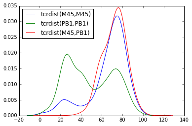
Code For Distribution of Distances
import matplotlib
import matplotlib.pyplot as plt
import seaborn as sns
%matplotlib inline


def epitope_to_epitope(e1,
                       e2,
                       clone_df = tr.clone_df,
                       paired_tcrdist = tr.paired_tcrdist,
                       var = "epitope"):
  """
  A function for subsetting distances to TCRs with shared or distinct or
  shared epitope specificity.
  """
  e1_ind = clone_df[var] == e1
  e2_ind = clone_df[var] == e2
  tr_df = pd.DataFrame(paired_tcrdist)
  e1_to_e2 = tr_df.loc[e1_ind , e2_ind].values.flatten()
  return(e1_to_e2)

sns.kdeplot(epitope_to_epitope(e1 = "M45", e2 = "M45"), bw = 4, label = "tcrdist(M45,M45)")
sns.kdeplot(epitope_to_epitope(e1 = "PB1", e2 = "PB1"), bw = 4, label = "tcrdist(PB1,PB1)")
sns.kdeplot(epitope_to_epitope(e1 = "M45", e2 = "PB1"), bw = 4, label = "tcrdist(M45,PB1)")
plt.legend(loc = 2);